Plot probabilities as areas underneath the PDF

plot_probability(
  model,
  lower = NULL,
  upper = NULL,
  distribution = NULL,
  details = NULL,
  fill = "grey35",
  color = "grey35",
  alpha = 1,
  ...
)

Arguments

model	one of R's built-in probability distributions (e.g., 'rnorm', 'rpois', 'runif').
lower	lower bound of P(a <= x <= b), i.e. b. Defaults to NULL.
details	details about the distribution (e.g., mean and sd). Used in the plot subtitle(s). Defaults to NULL.
fill	fill color of the histogram or density. Defaults to "grey35" (the ggplot2 default)
alpha	transparency of the histogram or density. Defaults to 1 (no transparency)
...	additional arguments passed to `model` (e.g. mean and sd for `rnorm`, lambda for `rpois`, etc.)
uppder	upper bound of P(a <= x <= b), i.e. a. Defaults to NULL.
density	plot the kernel density estimates instead of the histogram. Defaults to FALSE.
name	name of the distribution (a string). Used in the plot title(s). Defaults to NULL, in which case `model` is used in the plot title.

Value

ggplot object

Note

Should this function merge with `plot_distribution()`?

Author

Lawrence R. De Geest

Examples

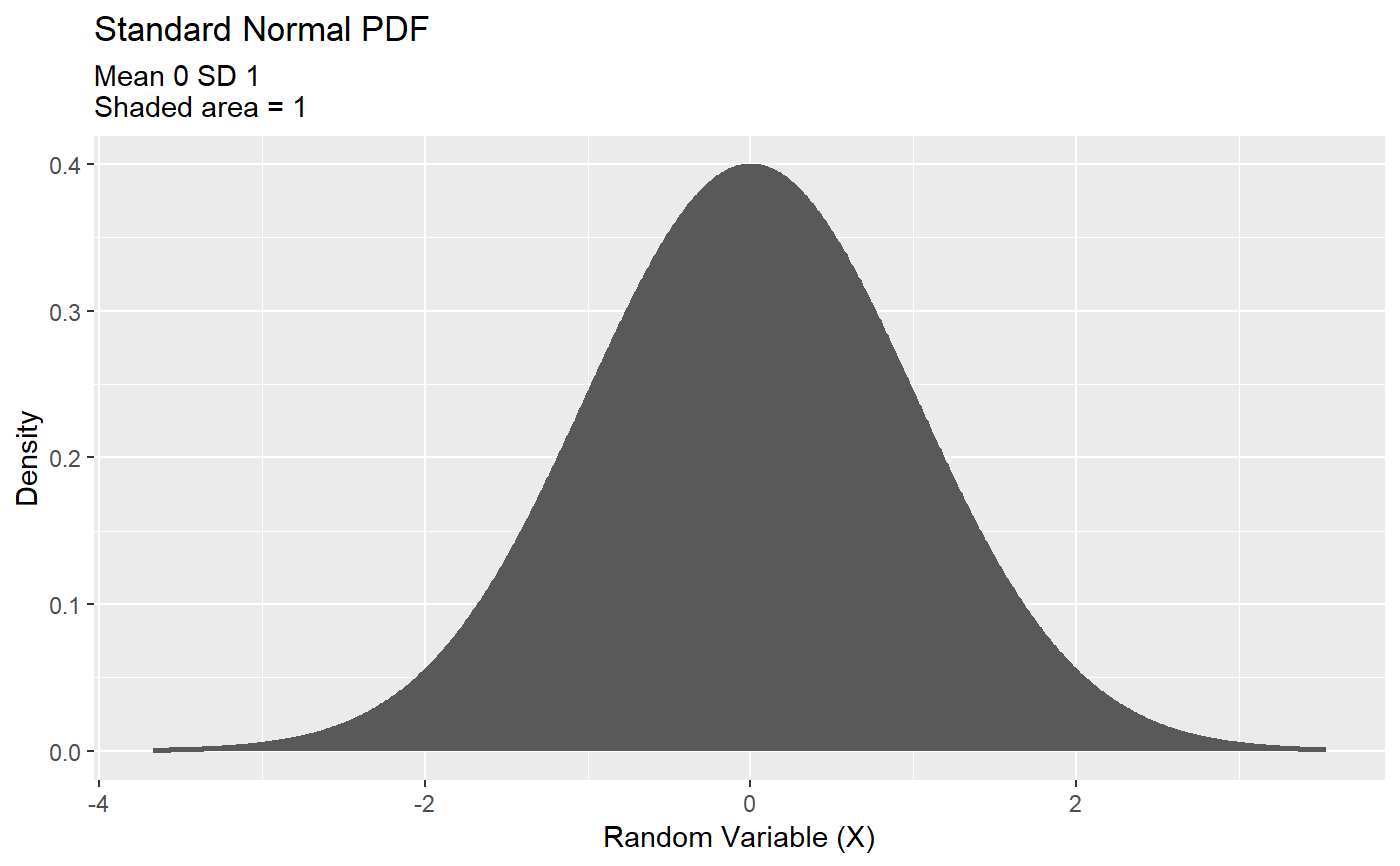
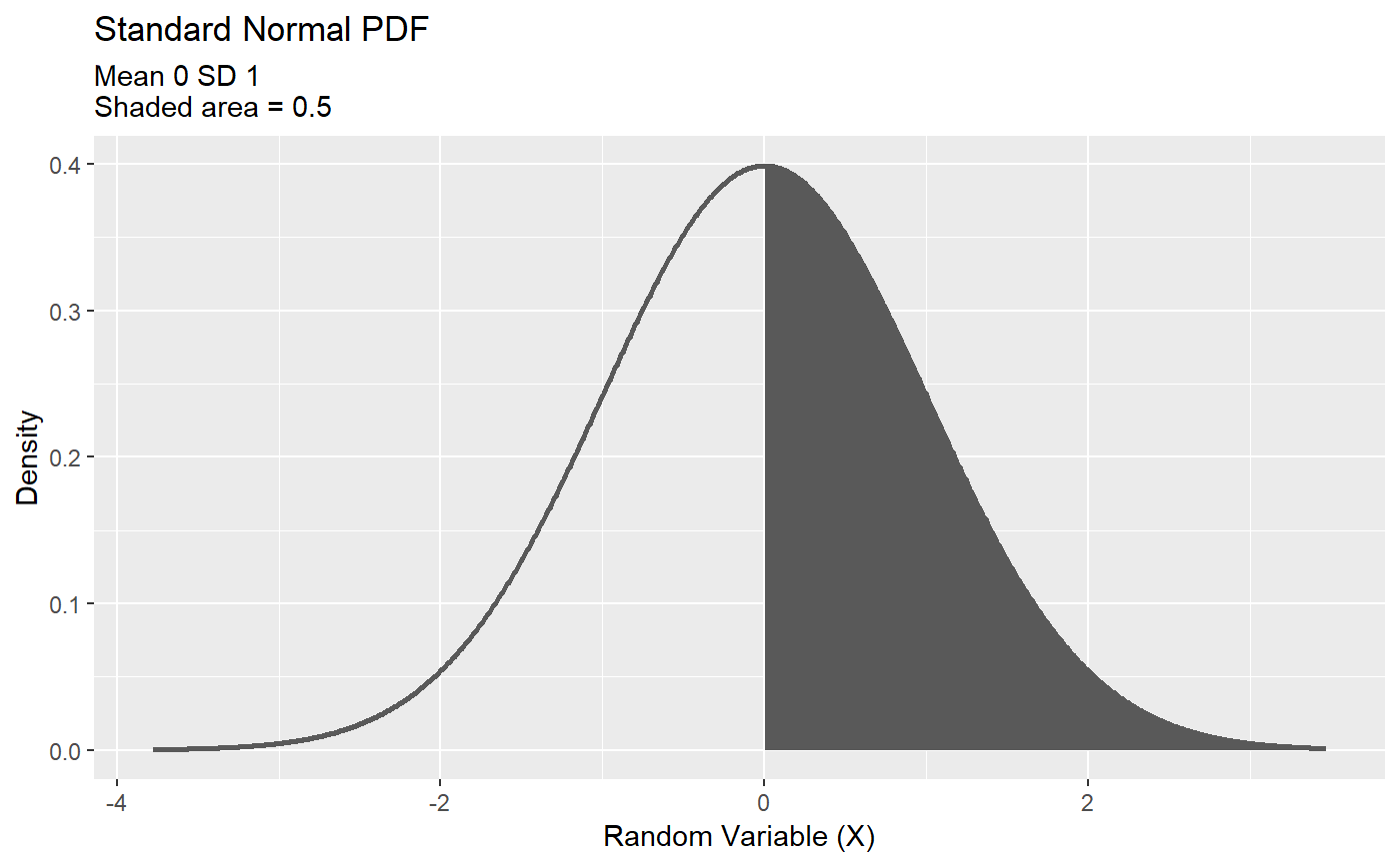
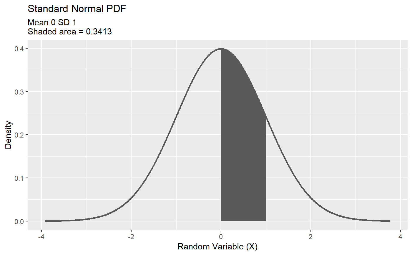
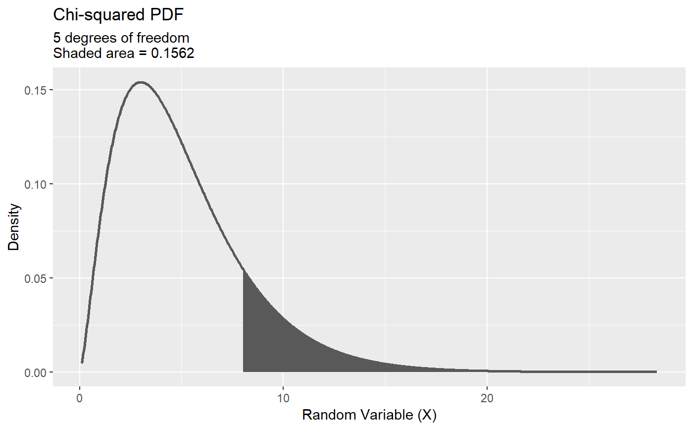
# plot the standard normal and show the entire distribution sums to 1
plot_probability(model = 'rnorm', lower = -Inf, distribution = "Standard Normal", details = "Mean 0 SD 1")

# ...and half the distribution sums to 0.5
plot_probability(model = 'rnorm', lower = 0, distribution = "Standard Normal", details = "Mean 0 SD 1")

# show the area between 0 and 1 on the standard normal
plot_probability(model = 'rnorm', lower = 0, upper =1,  distribution = "Standard Normal", details = "Mean 0 SD 1")

# Chi-squared distribution with 5 degrees of freedome
plot_probability(model = 'rchisq', df = 5, lower = 8, distribution = "Chi-squared", details = "5 degrees of freedom")