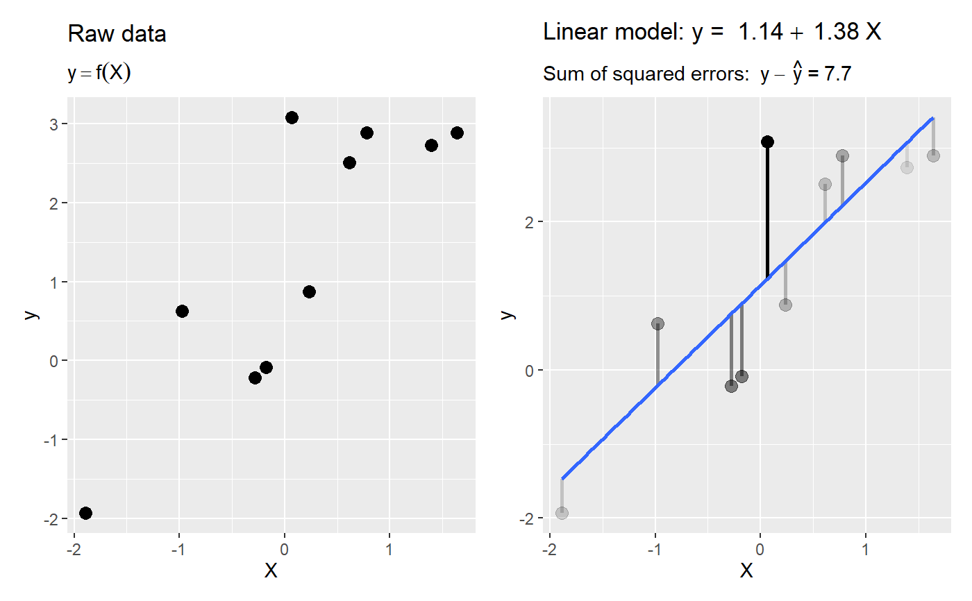
Simple demo of OLS

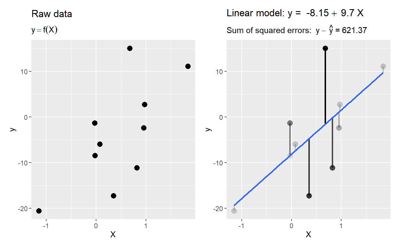
Plot a random scatter of Y and X variables, then plot the OLS line with errors

plot_ols(
  n = 10,
  betas = c(intercept = 1, slope = 1),
  x = c(mean = 0, sd = 1),
  error = c(mean = 0, sd = 1),
  seed = NULL,
  show_raw_data = TRUE,
  ...
)

Arguments

n	number of observations. Defaults to 10 (smaller `n` is easier to visualize).
betas	vector of coefficients (intercept and slope). Defaults to c(intercept = 1, slope = 1)
x	vector of parameters of the normal distribution of the independent variable. Defaults to c(mean = 0, sd = 1)
error	vector of parameters of the normal distribution of the error term. Defaults to c(mean = 0, sd = 1)
seed	seed for the random number generator. Defaults to NULL (i.e., varies each time you run it)
show_raw_data	plot the raw data alongside the plot with the regression line. Defaults to TRUE

Value

ggplot object if plot = TRUE, otherwise a data.frame

Author

Lawrence R. De Geest

Examples

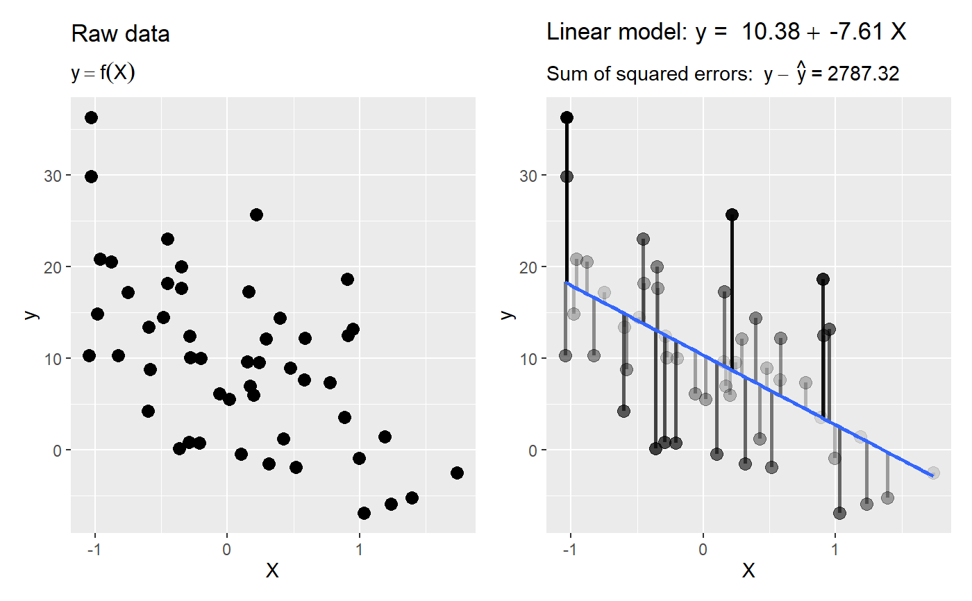
# default values are probably sufficient to the the main idea across
plot_ols()

# add some noise
plot_ols(error = c(mean = 0, sd = 10))

# add some more points and make the relationship negative
plot_ols(n=50, betas = c(intercept = 10, slope = -5), error = c(mean = 0, sd = 10))